First a Story

You are looking for a job, and you receive two job offers. One is 200K$ a year, and the second is 100K$ + stock options. Which is better? “Well Nivge” you’d tell me, “it depends on the value of the options and the probability they will liquidate”. That’s true, so let’s assume that there is a 10% chance they will be worth 1M$ (a year), and a 90% chance they (the stock options) will be worthless. Now, what do you prefer?

In this post I’ll show why the diminishing return of money should make you more “risk-averse” (preferring higher certainty alternatives), and why the 10% for 1M$ is more equivalent to a definite 25K$, rather than 100K$ which is the expected payout (=10%*1M$).

Diminishing Returns of Money

Most people would agree that money has a diminishing return kind of dynamic. Meaning, +10K$ would add more to your happiness if you were broke than if you were a millionaire. This is simple and has some interesting consequences when comparing financial opportunities with different uncertainties.

But first, how much does the return from money actually diminish?

Several studies show slightly different results, but the effect seems to be logarithmic, which means that for happiness on a scale of 1 to 10, you achieve roughly 0.5 points for every doubling of your income. This is why the richer you are, the more money you need for the same happiness boost.

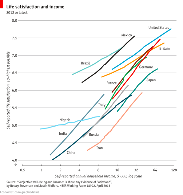
Look at one happiness measure, “life satisfaction”, vs annual income:

Note that the x-axis is in logarithmic scale (doubles every unit), so the relation looks linear, which means constant increase in satisfaction for every doubling of income (rather than for every constant increase in money – which is a “constant return” dynamic).

From this graph we have 3 main takeaways:

1. Countries have very different intercepts, meaning different satisfaction for the same annual income. Expected.
   1. For be example in an annual income of 16K$, happiness varies widely from 5 points in Iran to more than 7 in Brazil.
2. The relation in log scale is linear in all countries. Nice.
3. Most countries have a similar slope. Somewhere between 0.4 and 0.6. Even nicer.

The formula we derived to represent the relation between happiness and income is the following, where H stands for happiness, while m stands for money (in k$).

H(m)=H_0+r\cdot log(m)

r is the reward for doubling your income, we’ll use 0.5 as we’ve mentioned). H_0 is your happiness at 1K$ a year. We’ll take H_0 = 4.

The Effect of Uncertainty

When we are faced with comparing financial opportunities, we often have to account for uncertainty. Comparing a certain (meaning no uncertainty) earning of 100K$ to 200K$ is trivial (in the financial aspect). But comparing a certain earning of 100K$ to a 10% chance to win a 1M$ is not trivial.

It is common to compare expectancies (averages) in the presence of uncertainty, and somewhat justified by the laws of big numbers – over many decisions the sum of outcomes will converge to the sum of expectancies. So in the former case, the two options would be equivalent (average of 100K$).

The reason this is not accurate is that what people are actually interested in is maximizing their total happiness (rather than their total money). Even though money and happiness, are monotonically increasing (one goes up, the other also goes up), their expectancies are not maximized together due to the diminishing returns of money. Meaning different financial options maximize different targets (money or happiness).

So let’s compare the expected amount of happiness between a certain 200K$ and a 100K$+ 10% chance to earn a 1M$.

1. 100K$ + stocks

In the stock options case, we have a 90% chance to earn 100K$, and a 10% chance to earn 1.1M (=100K+1M$). To calculate the expected happiness of this opportunity we can calculate the happiness for each of the outcomes, and do a weighted average with their respective probabilities. Let’s go.

From formula #1 (there’s only one=]):

1. The happiness for the 100K$ outcome is 4+0.5*log(100), which is 7.32.
2. The happiness for 1.1M outcome is 4+0.5*log(1100) which equals 9.05

So the weighted average is: 90%*7.32+10%*9.05 = 7.49.

So to sum up, the expected happiness from the 100k$+ stocks is 7.49. Not bad. Next will see how it compares to the “no uncertainty opportunity”.

2. 200K$

Now, the happiness for this opportunity is simple. There’s just one outcome which is 200K$, so it’s corresponding happiness is 4+0.5*log(200) which equals 7.82.

Well that’s larger than the 7.49 of the stocks options.

Interesting. That means that although both options have the same expected money, They don’t have the same expected happiness.

Comparable Certain Salary

So now the inevitable question is what certain salary would give us the same expected happiness as the stocks option (=7.49)?

Turns out to be 127K$. Now if I lost you in the logarithms calculations that’s fine, now is the time to bounce back because the next sentence sums up the main thesis:

That means that in terms of happiness, a 10% chance to earn 1M$ is worth 27K$ (much less than the 100K$ that is the average amount of money).

So due to uncertainty we have, what we’ll call a ”happiness equivalence factor” from the average, of 27% (27K$/100K$).

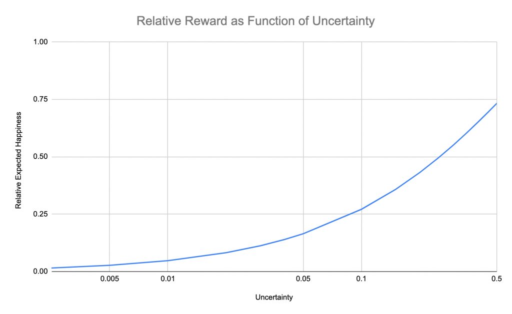
As you might have guessed, this happiness equivalence factor will be smaller the higher the uncertainty. How much you ask? Great question, here’s a graph:

This graph shows you how much you need to multiply the expected (average) sum of money, to get the equivalent certain money that would give you the same expected happiness.

Let’s look at three opportunities, all with expected amount of 100K$, but different uncertainties:

1. 50% to earn 200K$ will give a happiness equivalence factor of 73%. You get this by taking the graph at 0.5 (=50%). So equivalent to 73K$.

2. 10% chance to earn 1M$ will give a happiness equivalence factor of 27%, as we already saw earlier.

3. And if you have a 1% chance to earn 10M$, the factor is 4.7%(!) (graph at 0.01) which means that a 1% chance to earn 10M$ is worth a certain 4.7K$ (and not the average 100K$!)

That’s crazy.

Now, who wants to start a startup?

-Nivge

Subscribe to the newsletter.